Introduction
If you haven’t read the previous articles, I really encourage to start from the beginning, EXPLAIN can seem a bit complicated if you don’t have the basics. So don’t hesitate to take a look at the first and second article on the subject. Moreover reading them will give you the data model and a bit more information on the examples used here !
But if you have read them, welcome back !
Now that you’re a bit more familiar with EXPLAIN, the notions of costs, actual times, the different algorithm of scans, let’s talk about joining tables.
Nested loops
Let’s take a simple example, I want to get my owls with their jobs, for only the first jobs in my table.
So I do the following
owl_conference=# EXPLAIN ANALYZE SELECT * FROM owl JOIN job ON (job.id = owl.job_id)
                 WHERE job.id < 3;
                 QUERY PLAN
------------------------------------------------------------------------------------
 Nested Loop  (cost=0.00..481.17 rows=2858 width=56)
              (actual time=0.021..12.661 rows=9002 loops=1)
   Join Filter: (owl.job_id = job.id)
   Rows Removed by Join Filter: 11002
   ->  Seq Scan on owl  (cost=0.00..180.02 rows=10002 width=35)
                        (actual time=0.011..1.875 rows=10002 loops=1)
   ->  Materialize  (cost=0.00..1.10 rows=2 width=21)
                    (actual time=0.000..0.000 rows=2 loops=10002)
         ->  Seq Scan on job  (cost=0.00..1.09 rows=2 width=21)
                              (actual time=0.006..0.007 rows=2 loops=1)
               Filter: (id < 3)
               Rows Removed by Filter: 5
 Planning time: 0.386 ms
 Execution time: 13.324 ms
(10 rows)
To perform a join, this Nested Loops algorithm loops on the owls, and for each owl, it loops over the jobs and joins on the owl.job_id column.
If I wrote a nested loop in Python, it would be something like
jobs = Job.objects.all()
owls = Owl.objects.all()

for owl in owls:
    for job in jobs:
        if owl.job_id == job.id:
            owl.job = job
            break
The complexity being O(n*m), you can imagine how slow it could get on big tables.
Hash join
Let’s try to join on a little bit more rows.
owl_conference=# EXPLAIN ANALYZE SELECT * FROM owl JOIN job ON (job.id = owl.job_id)
                 WHERE job.id > 3;
                 QUERY PLAN
------------------------------------------------------------------------------------
 Hash Join  (cost=1.15..290.12 rows=7144 width=56)
            (actual time=0.143..4.790 rows=799 loops=1)
   Hash Cond: (owl.job_id = job.id)
   ->  Seq Scan on owl  (cost=0.00..180.02 rows=10002 width=35)
                        (actual time=0.032..2.258 rows=10002 loops=1)
   ->  Hash  (cost=1.09..1.09 rows=5 width=21)
             (actual time=0.082..0.082 rows=4 loops=1)
         Buckets: 1024  Batches: 1  Memory Usage: 9kB
         ->  Seq Scan on job  (cost=0.00..1.09 rows=5 width=21)
                              (actual time=0.020..0.024 rows=4 loops=1)
               Filter: (id > 3)
               Rows Removed by Filter: 3
 Planning time: 0.501 ms
 Execution time: 4.927 ms
(10 rows)
To perform a hash join:
- A hash table is created in memory with the join values and a pointer to the rows.
- This hash is used to join
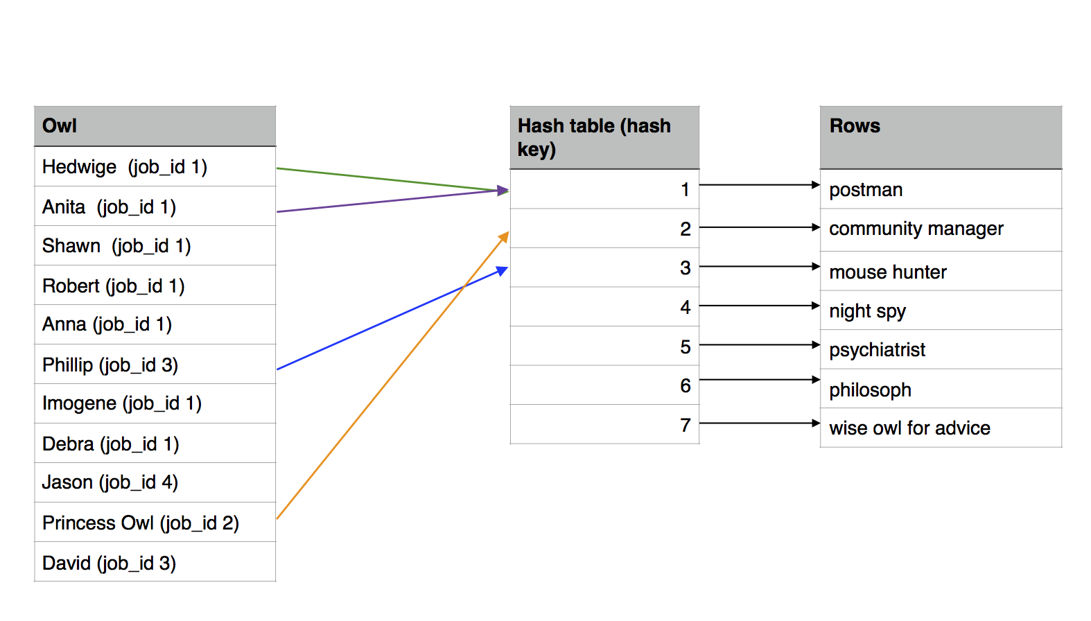
For the Python developers, it would be like creating a dictionnary for the job table. Like this:
jobs = Job.objects.all()

jobs_dict = {}
for job in jobs:
    jobs_dict[job.id] = job

owls = Owl.objects.all()
for owl in owls:
    owl.job = jobs_dict[owl.job_id]
This is much more efficient than the nested loop isn’t it? So why isn’t it used all the time ?
- For small tables, the complexity of building the hash table makes it less efficient than a nested loop.
- The hash table has to fit in memory (you can see it with
Memory Usage: 9kBin theEXPLAIN), so for a big set of data, it can’t be used. The same way you wouldn’t create a dictionnary containing 1M values.
Merge join
If neither Nested Loop or Hash Join can be used for joining big tables, what is the algorithm used then?
I am here joining the letters (about 400 000 rows) with the human table on the receiver_id column. So basically I want all the letters with their recipients, ordered by recipients.
owl_conference=# EXPLAIN ANALYZE SELECT * FROM letters JOIN human ON (receiver_id = human.id)
                 ORDER BY letters.receiver_id;
                                                            QUERY PLAN
----------------------------------------------------------------------------------------------------------------------------------
 Merge Join  (cost=55576.25..62868.63 rows=413861 width=51)
             (actual time=447.653..924.305 rows=413861 loops=1)
   Merge Cond: (human.id = letters.receiver_id)
   ->  Sort  (cost=895.22..920.25 rows=10010 width=23)
             (actual time=4.770..7.747 rows=10001 loops=1)
         Sort Key: human.id
         Sort Method: quicksort  Memory: 1167kB
         ->  Seq Scan on human  (cost=0.00..230.10 rows=10010 width=23)
                                (actual time=0.008..1.777 rows=10010 loops=1)
   ->  Materialize  (cost=54680.83..56750.14 rows=413861 width=24)
                    (actual time=442.856..765.233 rows=413861 loops=1)
         ->  Sort  (cost=54680.83..55715.48 rows=413861 width=24)
                   (actual time=442.793..687.048 rows=413861 loops=1)
               Sort Key: letters.receiver_id
               Sort Method: external merge  Disk: 15304kB
               ->  Seq Scan on letters  (cost=0.00..7582.61 rows=413861 width=24)
                                        (actual time=0.015..69.756 rows=413861 loops=1)
 Planning time: 0.587 ms
 Execution time: 982.440 ms
(13 rows)
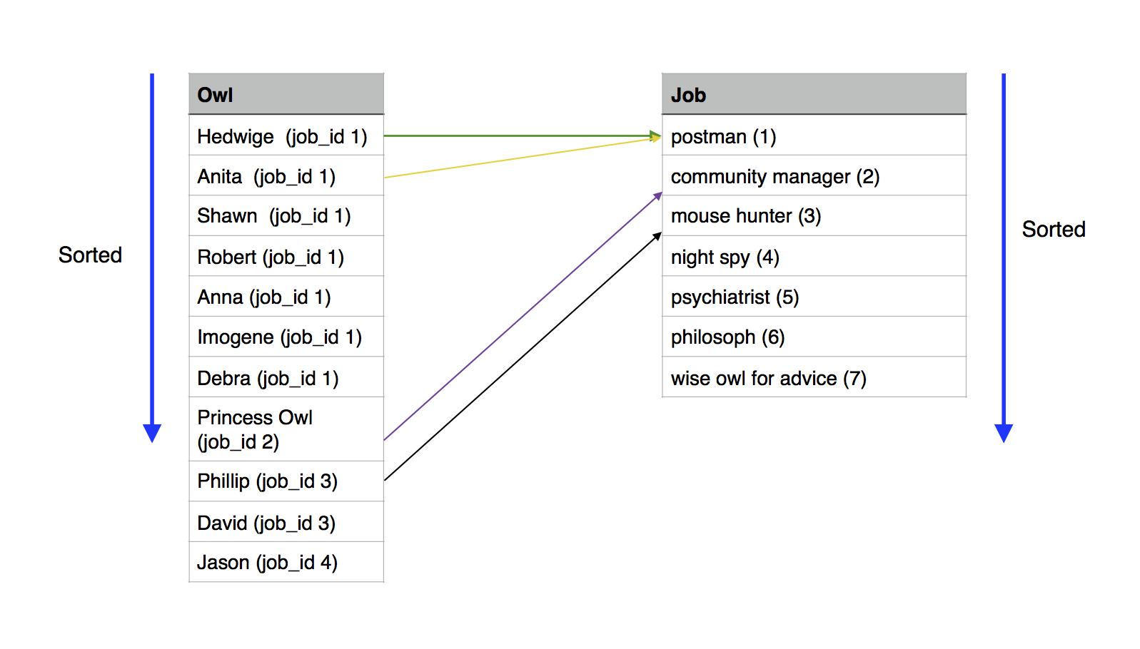
What you can see here is that it’s using a Merge Join. To do that:
- The two tables are sorted on the join value
- The join is performed on the sorted tables
This query takes almost a second and you can see that the quicksort (explained in the next article, that will be online in a couple days) uses Memory: 1167kB to sort the human table.
As for the letters table, it uses external merge Disk: 15304kB. That’s because I have a work_mem setting of 4MB that makes it impossible to sort directly in Memory.
If I added an index:
CREATE INDEX ON letters(receiver_id);
Then I would avoid sorting in Memory or on Disk.
owl_conference=# EXPLAIN ANALYZE SELECT * FROM letters JOIN human ON (receiver_id = human.id)
                 ORDER BY letters.receiver_id;
                 QUERY PLAN
----------------------------------------------------------------------------------------------
 Merge Join  (cost=0.71..31442.44 rows=413861 width=51)
             (actual time=0.033..648.119 rows=413861 loops=1)
   Merge Cond: (human.id = letters.receiver_id)
   ->  Index Scan using humain_pkey on human  (cost=0.29..1715.43 rows=10010 width=23)
                                              (actual time=0.005..4.766 rows=10001 loops=1)
   ->  Index Scan using letters_receiver_id_idx on letters  (cost=0.42..24530.28 rows=413861 width=24)
                                                            (actual time=0.024..502.212 rows=413861 loops=1)
 Planning time: 0.626 ms
 Execution time: 691.338 ms
(6 rows)
The query is still slow, so this is the kind of situation where you would have to wonder why you want 400 000 letters with their receivers… Who would really read that page ?
Conclusion
I hope that you enjoyed reading this article and that now, you feel familiar with costs, actual times, scans and joins.
The last step will be using ORDER BY and the serie of articles on EXPLAIN is over ! So here it is :)